Titanic Data

We take a look at the titanic dataset.

What variables contributed to an individuals survival?

Did different ages or sexes have a higher rate of survival?

Cleaning the data

We had two missing ages. We can replace that with the median.

# Replacing missing ages with median df['Age'] = df['Age'].fillna(df['Age'].median())

The cabin data had very little data. We drop that.

# Delete Cabin del df['Cabin']

We drop the remaining rows that have NaN's.

# Drop remaining NaN's df.dropna(inplace=True)

Plotting the data

I started by plotting all peoples ages and their survival.

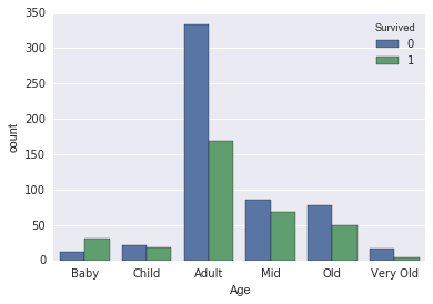
Age	Category
0-5	Baby
6-15	Child
16-30	Adult
31-40	Mid
41-60	Old
61-80	Very Old

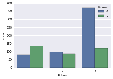
I then plotted each class and their survival.

This is a a little difficult to read. Why dont we put it into a stacked bar graph to see the weight of each genre and the songs in that genre hitting Number 1.

Data Wrangling

In an attempt to figure out which coefficients I should use, I normalized the appropriate data and ran a RFE model.

nc = [x for x in df.columns if x not in ['Survived', 'Sex', 'Embarked', 'index', 'PassengerId' , 'Name', 'Ticket']] df_norm = (df[nc] - df[nc].mean()) / (df[nc].max() - df[nc].min()) svc = SVC(kernel="linear", C=1) rfe = RFE(estimator=svc, n_features_to_select=1, step=1) rfe.fit(df_norm, df.Survived) ranking = rfe.ranking_ coeffs = pd.DataFrame(ranking, index=df[nc].columns, columns=['coef']) coeffs.sort_values('coef')

	coef
Pclass	1
Fare	2
Age	3
SibSp	4
Parch	5

I dropped the fare data since the class data can represent similar findings but with a higher correlation.

Created dummy vriables for:

Sex
Age (binned with the table above)
Embarked
Pclass

Regression

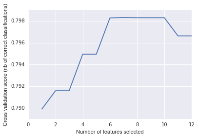
I ran a RFECV to figure out the optimal number of features to use to get the highest score. What I figured out was that 7 features was the best

So I ran a Logistic Regression and received these absolute coefficients.

	Coefficient	Feature
2	2.600351	male
5	2.032660	Age_Baby
10	1.482869	Class_1
11	0.908808	Class_2
3	0.585350	Embark_C
0	0.447184	SibSp
6	0.365025	Age_Child
9	0.180293	Age_Old
4	0.161709	Embark_Q
1	0.072917	Parch
8	0.049452	Age_Mid
7	0.044070	Age_Adult

Since 4 of the bottom 5 coefficients are dummy created variables, we can only drop the Parch variable from our model.

With the new model, we end up with this confusion matrix

	Predicted Survived	Predicted did_not_survive
Survived	82	30
Did not Survive	26	156

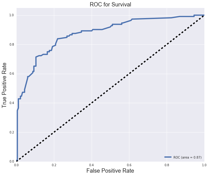
With an roc curve:

We try the model with a GridSearch, we end up with this confusion matrix

	Predicted Survived	Predicted did_not_survive
Survived	80	32
Did not Survive	25	157

We perform a Gridsearch for the same classification problem as above, but use KNeighborsClassifier a our estimator. The best parameters end up being

{'n_neighbors': 3, 'weights': 'uniform'}. So we fit a new kNN model with the optimal parameters found in gridsearch and end up with this confusion matrix.

	Predicted Survived	Predicted did_not_survive
Survived	75	37
Did not Survive	30	152

Which turns out to be worse than our original Linear model.

Perhaps it's better to keep our model linear.

Hope you enjoy my findings :)