We scraped all the salary data from glassdoor for data scientists across all US cities using a custom script running Selenium Webdriver and BeautifulSoup.
Which city has the highest paying salaries?
Do different cities value Data Scientist salries more than others?
Does a company's field have any correlation with Data Scientist Salaries?
Cleaning the data
The stock data is cleaned for: Certain terms in the name. Things like 'inc,' or 'corp' are deleted. This helps the matching process. The market cap information is converted from strings to millions of dollars.
The city data is cleaned for: Cities containing '-' Cities containing 'county' Removing ',' from city names
We had discrepancies between the names of the scraped Glass Door data, and the names of the stock information. This led to information not being merged when it should have. So, we manually searched for the pairs of names and input them into a dictionary. This dictionary would be used to rename the mislabeled Glass Door entries.
We initiate a Glass Door data frame to connect the json to. We upload the json, which has four columns:
- Location
- Company
- Salary
- Job
We end up with this table head
| Location | Company | Salary | Job | |
|---|---|---|---|---|
| 0 | Albany, NY | GE | 104000.0 | Data Scientist |
| 1 | Arlington, TX | State Farm | 105000.0 | Data Scientist |
| 2 | Arlington, TX | Epsilon | 166000.0 | Data Scientist |
| 3 | Arlington, TX | Match | 82000.0 | Data Scientist |
| 4 | Arlington, TX | Hudl | 90000.0 | Data Scientist |
This is our job title value counts
- Data Scientist 945
- Senior Data Scientist 375
- Principal Data Scientist 59
- Junior Data Scientist 38
- Entry Level Data Scientist 28
- Data Scientist II 18
- Data Scientist Intern 17
- Associate Data Scientist 16
- Data Scientist Intern - Hourly 15
- Data Scientist Intern - Monthly 11
- Data Scientist I 6
- Senior Data Scientist/Statistician 4
- Staff Data Scientist 3
- Clinical Laboratory Scientist-data Analyst 2
- Chief Data Scientist 2
- Scientist, Statistical and Data Sciences 2
- Data Visualization Scientist 2
- Lead Data Scientist 1
- Software Engineer (Data Scientist) 1
- Data Scientist - Hourly 1
We merge the glass_door df with stocks. We only select those Jobs that are Junior Level, Middle Level, or Senior Level. We dont want to end up with internships. We then bin the jobs with their respective bin names (as just mentioned). For the most recurring private companies, market cap and sectors were updated as they had an impact on prediction ability. Null values in market cap and sector were changed appropriately.
We end up with these job title value counts
- DS 929
- Senior DS 431
- Junior DS 91
We converted the most relevant columns to dummy variables. We played around with this a lot, and found that Sector, Region, Job, MarketCap, and various living index components contributed positively to our logistic regression. All other columns were deleted.
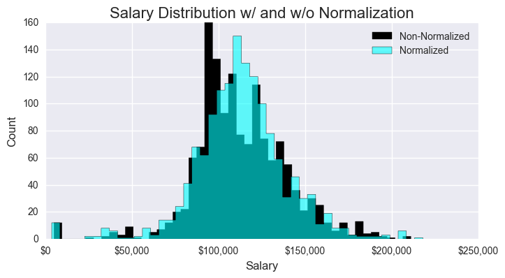
Additionally, we found that normalizing the salary data against the total living index helped to make the salary data gaussian. So, we also multiplied all of the independent variables against their corresponding living index.
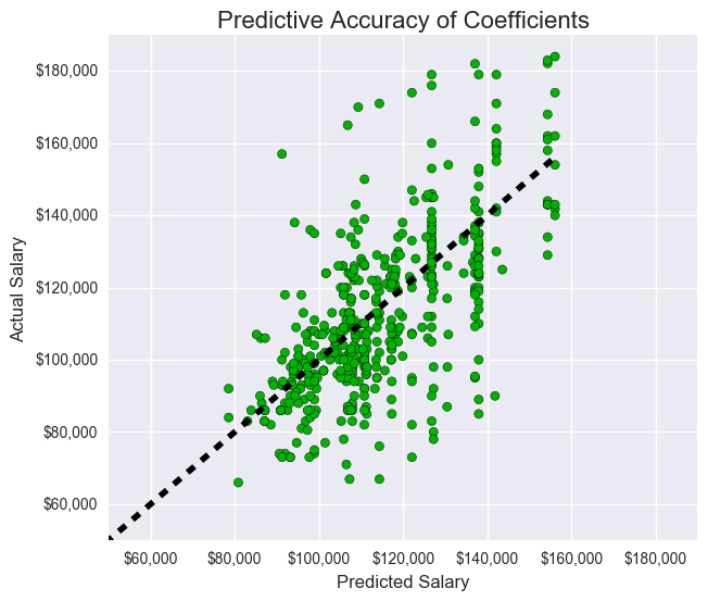
Regressing and plotting the Data
Below are plots demonstrating the strength of our coefficents and the normalization of our salaries.
We decided to run a normal regression on our variables to see their predictive power. We figured that reducing the variance would greatly help our ability to classify our outputs for the logistic regression.
For the logistic regression below, we found the optimal tunings for our logistic regression outputs by running a series of for loops to find the best calibrations parameters. Furthermore, we took the average of the precision, recall, and f1scores over the course of 20 different random_states to find a more fair score.
Best f1:   0.75
Best x0:   -1.5
Best x1:   0.9
Best x2:   -1.5
Number of bins:     3
Random Iterations:  5

Average Precision:  0.715619047619
Average Recall:     0.719666666667
Average F1-Score:   0.713952380952

Variance Precision: 6.84263038549e-05
Variance Recall:    0.000754650793651
Variance F1-Score:  0.00051533106576
               113000-162000  162000-211000  64000-113000
113000-162000            143              0            52
162000-211000             15              0             4
64000-113000              41              1           229
               precision    recall  f1-score   support

113000-162000       0.72      0.73      0.73       195
162000-211000       0.00      0.00      0.00        19
 64000-113000       0.80      0.85      0.82       271

  avg / total       0.74      0.77      0.75       485
Best f1: 0.75 Best x0: -1.5 Best x1: 0.9 Best x2: -1.5 Number of bins: 3 Random Iterations: 5 Average Precision: 0.715619047619 Average Recall: 0.719666666667 Average F1-Score: 0.713952380952 Variance Precision: 6.84263038549e-05 Variance Recall: 0.000754650793651 Variance F1-Score: 0.00051533106576 113000-162000 162000-211000 64000-113000 113000-162000 143 0 52 162000-211000 15 0 4 64000-113000 41 1 229 precision recall f1-score support 113000-162000 0.72 0.73 0.73 195 162000-211000 0.00 0.00 0.00 19 64000-113000 0.80 0.85 0.82 271 avg / total 0.74 0.77 0.75 485
The data below represent our trials on only Senior Data Scientist positions, but reflect upon how the model changes with subsequent changes in the input parameters. The best f1-score we obtained surprisingly did not use job dummy variables.
BEST with Junior Jobs and no Job Dummies
Number of bins: 3- Average Precision: 0.756315789474
- Average Recall: 0.754736842105
- Average F1-Score: 0.751052631579
Best with No Junior Jobs and Job Dummies
Number of bins: 3- Average Precision: 0.755789473684
- Average Recall: 0.754210526316
- Average F1-Score: 0.75
Best with No Junior Jobs and no Job Dummies
Number of bins: 3- Average Precision: 0.756315789474
- Average Recall: 0.754736842105
- Average F1-Score: 0.751052631579
Standard Company Changes:
Number of bins: 3- Average Precision: 0.748947368421
- Average Recall: 0.748947368421
- Average F1-Score: 0.744736842105
With Private Company changes:
Number of bins: 3- Average Precision: 0.755789473684
- Average Recall: 0.754210526316
- Average F1-Score: 0.75
With PC changes and no Job Dummies:
Number of bins: 3- Average Precision: 0.756315789474
- Average Recall: 0.754736842105
- Average F1-Score: 0.751052631579
Standard Company Changes:
Number of bins: 3- Average Precision: 0.748947368421
- Average Recall: 0.748947368421
- Average F1-Score: 0.744736842105
With Private Company changes:
Number of bins: 3- Average Precision: 0.755789473684
- Average Recall: 0.754210526316
- Average F1-Score: 0.75
With Private Company changes and Sector-MarketCap Bin:
Number of bins: 3- Average Precision: 0.753157894737
- Average Recall: 0.752105263158
- Average F1-Score: 0.748421052632
With PC changes and no State Dummies:
Number of bins: 3- Average Precision: 0.723684210526
- Average Recall: 0.726842105263
- Average F1-Score: 0.72
With PC changes and no Region Dummies:
Number of bins: 3- Average Precision: 0.754210526316
- Average Recall: 0.754210526316
- Average F1-Score: 0.748421052632
With PC changes and no Job Dummies:
Number of bins: 3- Average Precision: 0.756315789474
- Average Recall: 0.754736842105
- Average F1-Score: 0.751052631579
With PC changes, no J D, and no MarketCap Dummies
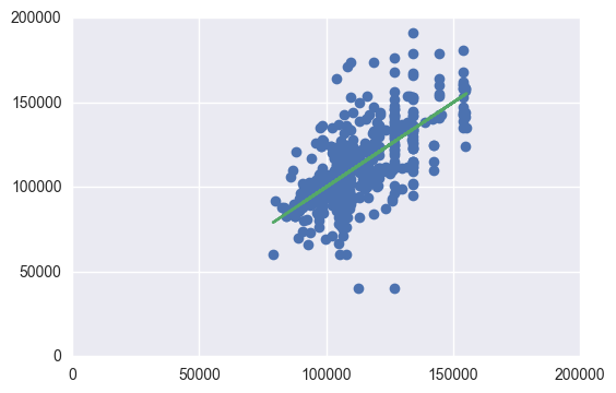
This is another regression on our input variables. It is of a different library, for added coefficient information. The x_train,y_train,... can be found just above the other regression graphs.
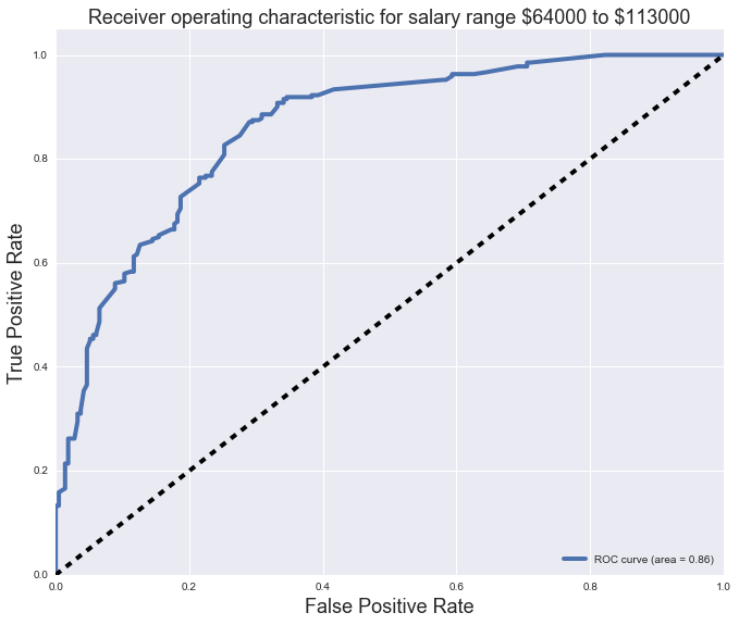
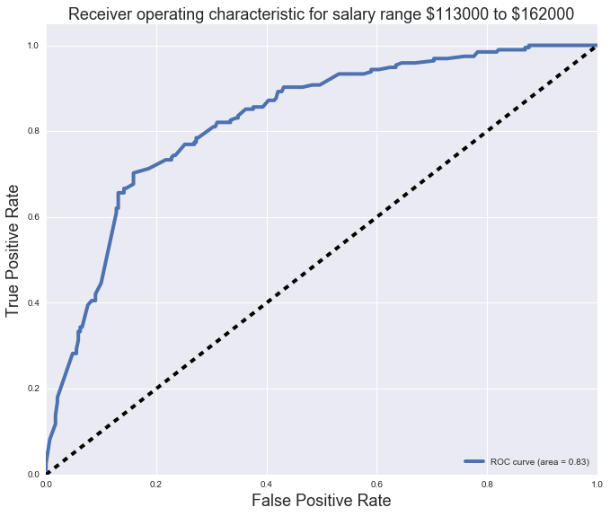
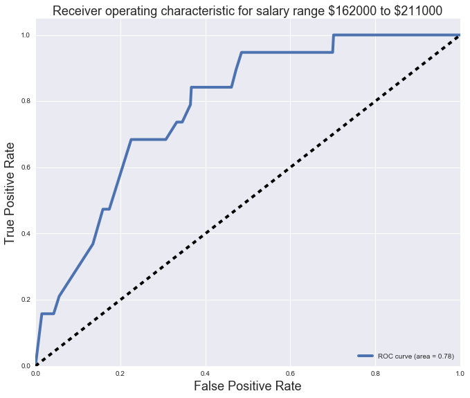
We then finally plot our ROC curves for each of the salary bins.
Hope you enjoy my findings :)
Collaborators: Thomas Voreyer, Jocelyn Ong,