We take a look at liquor sales in Iowa. We only took a 10% sample of the data as we found that to be a sufficient amount of data to look at (270,955 rows).
Which cities sell the most liquor?
Are some cities better served than others?
Where is the most under served city that we can open up a liquor store and compete?
Cleaning the data
This was our table data headers:
| Date | Store Number | City | Zip Code | County | Category | Category Name | Vendor Number | Item Number | Item Description | Bottle Volume (ml) | State Bottle Cost | State Bottle Retail | Bottles Sold | Sale (Dollars) | Volume Sold (Liters) | Volume Sold (Gallons) |
|---|
- We filled in missing values in County Names as well as misspelled city names.
- We fixed spelling errors.
- There were some values in the County field that did not parse correctly.
- We set individual values to the correct County.
- We filled in missing values in Category Names.
- We dropped the County Number column.
- We converted the Date column to datetime object.
- We dropped the Category column.
- We removed $ and converted appropriate columns to floats.
- We constrained the dataframe to 2015
- We created total cost column.
This was our new table:
| Store Number | Vendor Number | Item Number | Bottle Volume (ml) | State Bottle Cost | State Bottle Retail | Bottles Sold | Sale (Dollars) | Total_Cost | Volume Sold (Liters) | Volume Sold (Gallons) | |
|---|---|---|---|---|---|---|---|---|---|---|---|
| count | 218594.000000 | 218594.000000 | 218594.000000 | 218594.000000 | 218594.000000 | 218594.000000 | 218594.000000 | 218594.000000 | 218594.000000 | 218594.000000 | 218594.000000 |
| mean | 3578.700216 | 255.976783 | 45947.926064 | 925.621609 | 9.771547 | 14.675065 | 9.950456 | 130.503332 | 86.860051 | 9.087232 | 2.400800 |
| std | 942.194733 | 141.266301 | 52563.817681 | 492.014837 | 7.021363 | 10.531652 | 24.449269 | 386.612714 | 256.816527 | 29.360489 | 7.756215 |
| min | 2106.000000 | 10.000000 | 173.000000 | 50.000000 | 0.890000 | 1.340000 | 1.000000 | 1.340000 | 0.890000 | 0.100000 | 0.030000 |
| 25% | 2603.000000 | 115.000000 | 26828.000000 | 750.000000 | 5.510000 | 8.270000 | 2.000000 | 30.720000 | 20.430000 | 1.600000 | 0.420000 |
| 50% | 3715.000000 | 260.000000 | 38176.000000 | 750.000000 | 8.000000 | 12.300000 | 6.000000 | 70.560000 | 47.040000 | 5.250000 | 1.390000 |
| 75% | 4349.000000 | 380.000000 | 64573.000000 | 1000.000000 | 11.920000 | 17.880000 | 12.000000 | 135.660000 | 90.420000 | 10.500000 | 2.770000 |
| max | 9018.000000 | 978.000000 | 995507.000000 | 6000.000000 | 425.000000 | 637.500000 | 2508.000000 | 36392.400000 | 24261.600000 | 2508.000000 | 662.540000 |
Exploratory Data Analysis
Exploratory Data Analysis is performed to analyze the data for skewness, as well as build predictors for the target variable.
Bottles Sold, Sale (Dollars) are skewed. Plotting Histograms show that we should to restrict to Bottles Sold per transaction to 25 and less. This will eliminate outliers.
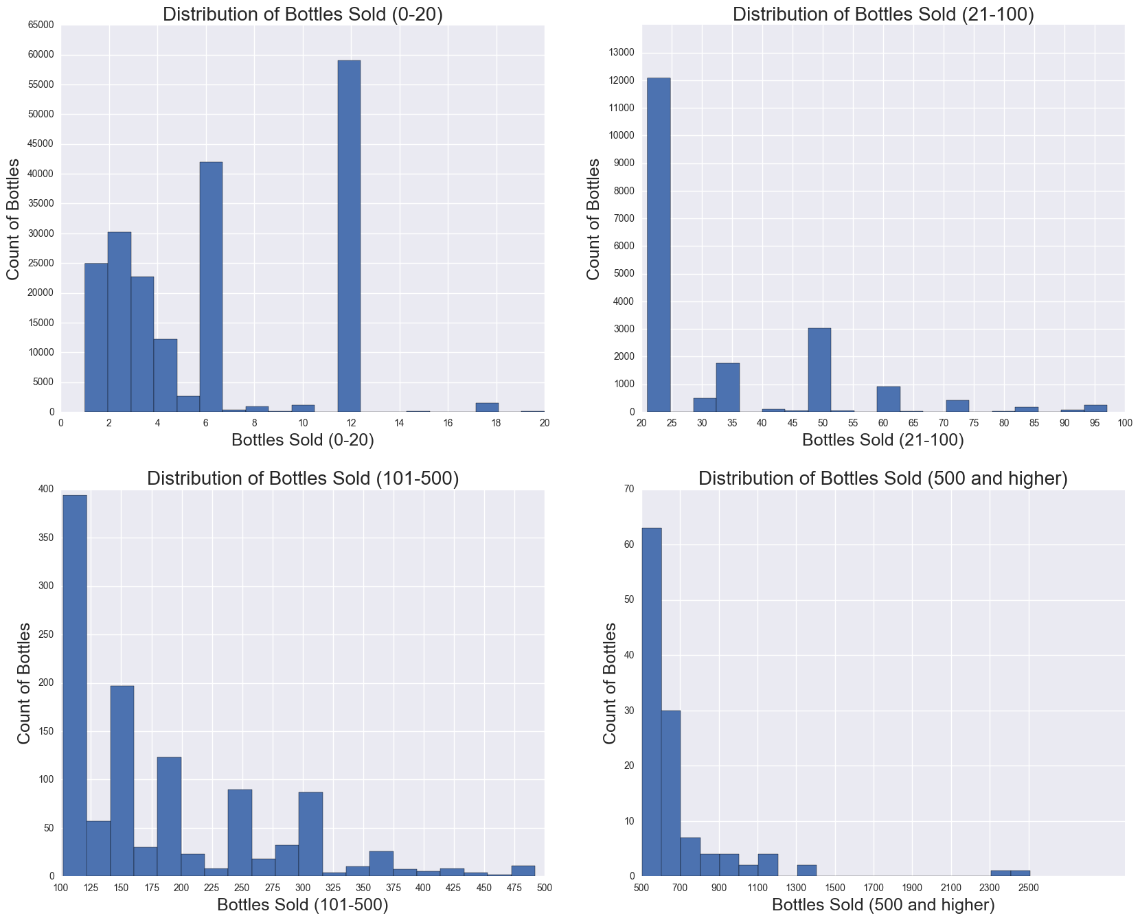
Only considering bottles sold 25 and under, because the percentage of transactions where Bottles Sold were 25 and under is: 96.06%. While the data is still skewed for Bottles Sold and Sale (Dollars), one standard deviation from the mean will not result in negative Bottles Sold and Sale (Dollars).
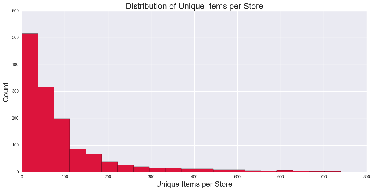
Unique Items per Store
By creating unique items per store, we can use it as a proxy for store size, which will one of the predictors used in the regression. The histogram for unique per items shows that it is skewed.
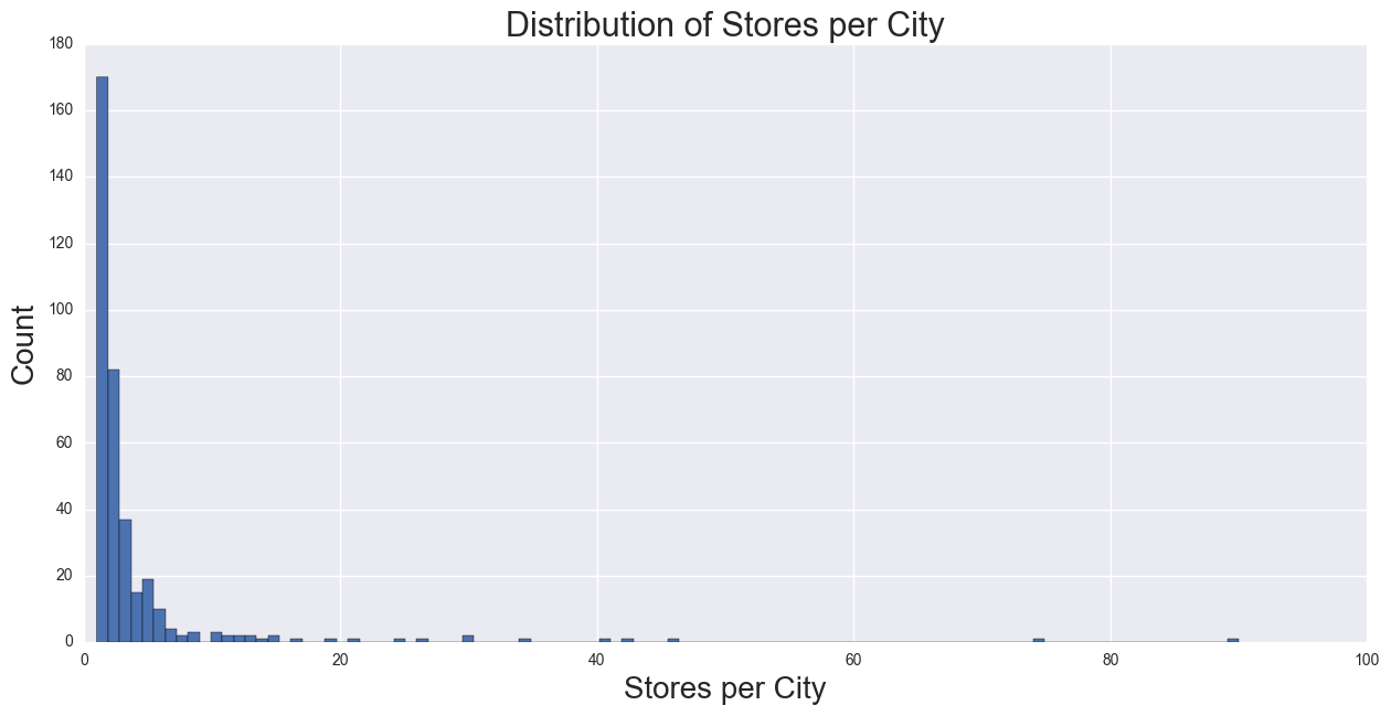
 Calculating the Number of Stores per City, which will be used for number of competitors as a predictor in the regression. From the histogram, the distribution is heavily skewed.
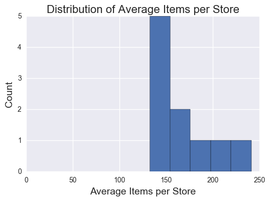
Average Items per Store per City
Calculating Average Items per Store per City and Sales per Store, which will be used later in merges. Histogram shows that there is a skewed distribution.
 Starting from the df (original) dataframe, and merging with various dataframes created prior, a dataframe is created to build metrics to be used as predictors for the regression, which are the following:
- Bottles Sold
- Items per Store
- Average Price
- Stores per City
- Population
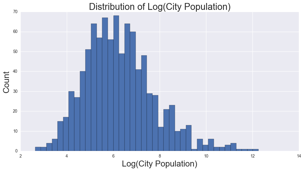
2015 Population by City
From the distribution of the histogram, Population by City is heavily skewed.
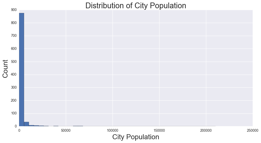 Taking the log normalizes the City Population Values. Predictors will be transformed by taking the log in the regression.
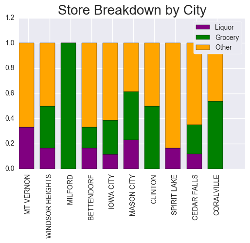
Categorizing the types of Liquor in the Data
By Categorizing the store name by whether it is a Liquor, Grocery, or Other, we can analyze the type of stores for the top 10 markets.
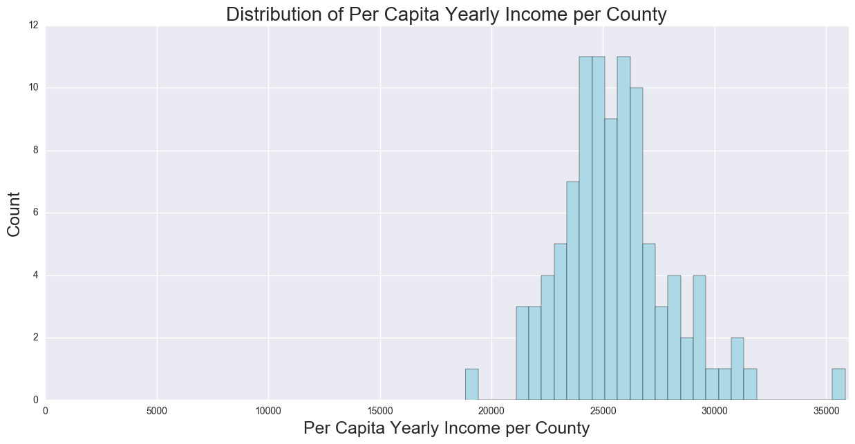
Final Additions:
Bringing in County-level Per Capita Yearly Income, to be used as a predictor for the regression. This distribution is still skewed, but less than other predictors.
Regression Analysis
The dataframe will be constructed to get the target (df_y) and the data for the predictors (df_X), which will then be split into train and test sets. The target variable is Bottles Sold. The predictors that will be used are the following: Target Variable: Yearly Bottles Sold (per each Store) Predictors:
- Items per Store
- Average Price
- Stores per City
- Population
- Per Capita Yearly Income
- Constraining the data to bottles sold per transaction to 25 and under
- Each store in a city is competing against each other
- Log-normalization due to the skewness of the target and predictors
- Per Capital Yearly Income, which is for county, is uniform across cities in the county
Our regression showed the following:
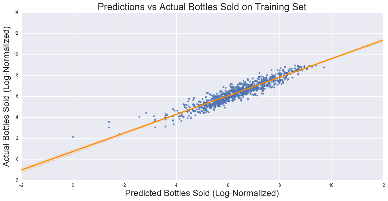
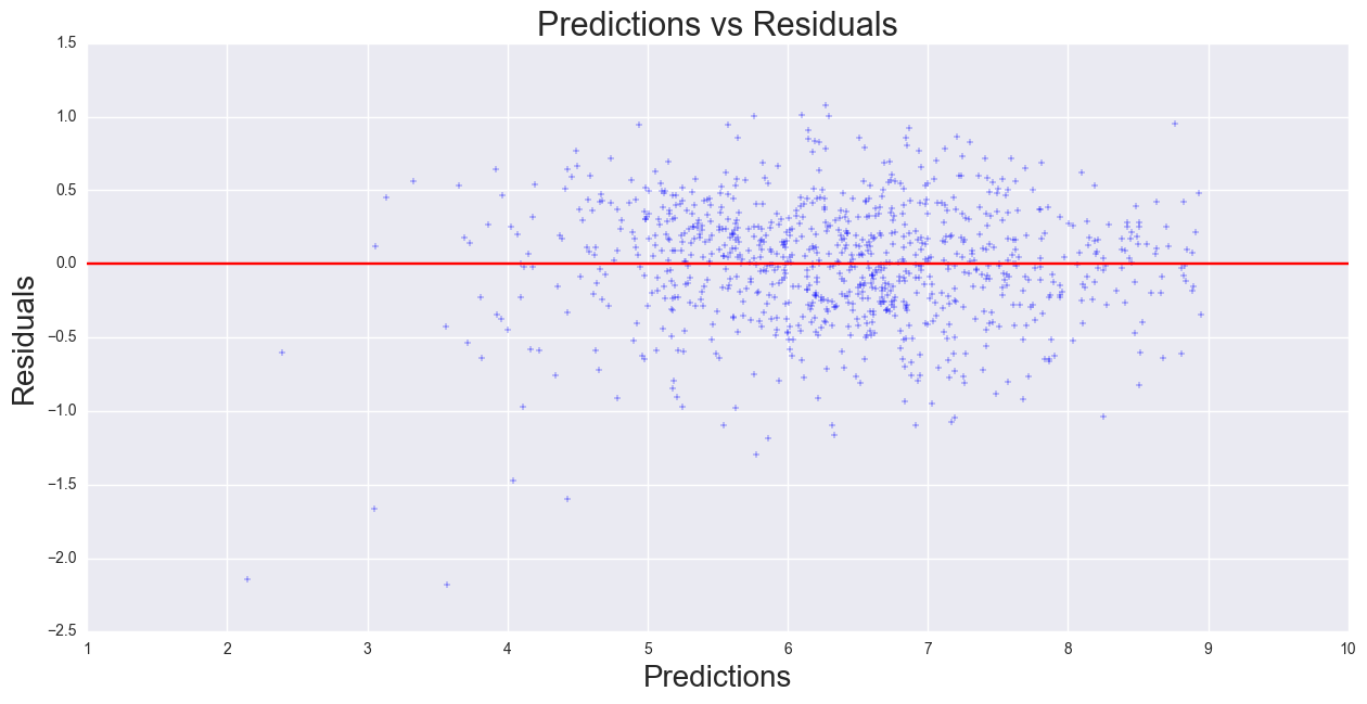
Analysis of the Results
The correlation on the training dataset is 0.88. The coefficients for the regression show the strongest predictor is Unique Items (positively correlated), followed by Average Price (negatively correlated), Stores per City/Number of competition (negatively correlated), and Population and Per Capital Yearly Income (both positively correlated). These relationships are what we expect to see: the number of items in a store would show that more available products to purchase, and as the number of competitors in the city as well as price should decrease the bottles sold. Population and Income should be positively correlated as the more people are in a city, the higher demand should be, and the more disposable income a person has, the more the person is able to spend on liquor. If the assumption of the Yearly per Capita Income is uniformly distributed across all cities in the county does not hold, then there would be a stronger bias, which requires city level Yearly per Capital Income.
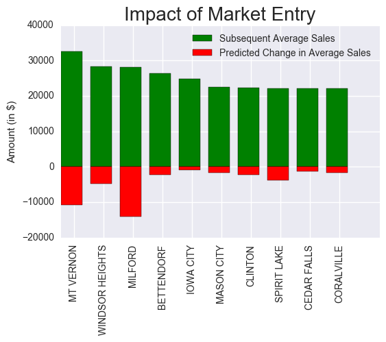
What happens if another store enters the market? Assuming Quantity (Bottles Sold per City) and Avg Price does not change (also means Total Sales (Dollars) per city does not change), if we increased number of stores per city by 1, we can calculate the new AvgSales with entry of a new store. Sorting from highest to lowest, we will find top 10 cities as consideration for markets to expand.
Once we know which markets to enter, we can find the average number of items among the competitors,types of competitors, and also the items and prices to which we place in the store.
| City | Total Sales (Dollars) | Number of Stores | Number of Stores + 1 | AvgSales | AvgSales_w_entry | Delta Sales% | Population | Liquor | Grocery | Other | Average_items_store | |
|---|---|---|---|---|---|---|---|---|---|---|---|---|
| 0 | MT VERNON | 130172.81 | 3.0 | 4.0 | 43390.936667 | 32543.202500 | -0.250000 | 4486 | 1 | 0 | 2 | 178.666667 |
| 1 | WINDSOR HEIGHTS | 198687.11 | 6.0 | 7.0 | 33114.518333 | 28383.872857 | -0.142857 | 4889 | 1 | 2 | 3 | 199.000000 |
| 2 | MILFORD | 84245.46 | 2.0 | 3.0 | 42122.730000 | 28081.820000 | -0.333333 | 3018 | 0 | 2 | 0 | 241.000000 |
| 3 | BETTENDORF | 343749.94 | 12.0 | 13.0 | 28645.828333 | 26442.303077 | -0.076923 | 35505 | 2 | 2 | 8 | 132.416667 |
| 4 | IOWA CITY | 670082.63 | 26.0 | 27.0 | 25772.408846 | 24817.875185 | -0.037037 | 74220 | 3 | 7 | 16 | 151.615385 |
| 5 | MASON CITY | 314249.36 | 13.0 | 14.0 | 24173.027692 | 22446.382857 | -0.071429 | 27366 | 3 | 5 | 5 | 155.692308 |
| 6 | CLINTON | 245612.03 | 10.0 | 11.0 | 24561.203000 | 22328.366364 | -0.090909 | 26064 | 0 | 5 | 5 | 136.200000 |
| 7 | SPIRIT LAKE | 155668.34 | 6.0 | 7.0 | 25944.723333 | 22238.334286 | -0.142857 | 5018 | 1 | 0 | 5 | 147.500000 |
| 8 | CEDAR FALLS | 399731.96 | 17.0 | 18.0 | 23513.644706 | 22207.331111 | -0.055556 | 41255 | 2 | 4 | 11 | 163.882353 |
| 9 | CORALVILLE | 308774.21 | 13.0 | 14.0 | 23751.862308 | 22055.300714 | -0.071429 | 20608 | 0 | 7 | 6 | 137.384615 |
* The store type has been incorporated to show the types of stores in a given city
The cities above are either subarbs (Windsor Heights, Bettendorf, Coralville), college towns (Mt. Vernon, Iowa CityCedar Falls, or near a resort/lake (Spirit Lake, Milford, Mason City). Categorizing the Category Name to bins of liquor types, we can find the ideal mix of inventory using the average items per store, which was calculated above (164 items per store) Evaluating the Predicted Sales (Predicted Bottles * Avg Price), we can re-run the same process to evaluate top 10 cities for Predicted Sales. Below, there are 7 Cities that are in the list above:
- Windsor Heights
- Cedar Falls
- Milford
- Iowa City
- Mt. Vernon
- Mason City
- Coralville
- Ames (college town)
- Monticello (rural iowa)
- Clear Lake (resort, next to Mason City)
- Windsor Heights
- Cedar Falls
- Milford/Spirit Lake
- Iowa City/Coralville
- Mason City/Clear Lake
Evaluating Predicted Sales (Predicted Bottles * Avg Price)
| City | Pred_Sales | Number of Stores | Number of Stores + 1 | Pred_AvgSales | Pred_AvgSales_w_entry | Average_items_store | |
|---|---|---|---|---|---|---|---|
| 0 | WINDSOR HEIGHTS | 172124.572356 | 6.0 | 7.0 | 28687.428726 | 24589.224622 | 199.000000 |
| 1 | CEDAR FALLS | 407049.343987 | 17.0 | 18.0 | 23944.079058 | 22613.852444 | 163.882353 |
| 2 | MILFORD | 67756.119496 | 2.0 | 3.0 | 33878.059748 | 22585.373165 | 241.000000 |
| 3 | IOWA CITY | 604113.134410 | 26.0 | 27.0 | 23235.120554 | 22374.560534 | 151.615385 |
| 4 | AMES | 580593.170325 | 25.0 | 26.0 | 23223.726813 | 22330.506551 | 149.440000 |
| 5 | MT VERNON | 86766.312096 | 3.0 | 4.0 | 28922.104032 | 21691.578024 | 178.666667 |
| 6 | MASON CITY | 291187.129485 | 13.0 | 14.0 | 22399.009960 | 20799.080678 | 155.692308 |
| 7 | MONTICELLO | 61698.954649 | 2.0 | 3.0 | 30849.477325 | 20566.318216 | 241.000000 |
| 8 | CORALVILLE | 272995.830038 | 13.0 | 14.0 | 20999.679234 | 19499.702146 | 137.384615 |
| 9 | CLEAR LAKE | 136262.829544 | 6.0 | 7.0 | 22710.471591 | 19466.118506 | 155.166667 |
Liquor Categories
Earlier, we created category bins to be used for our portfolio. We then further categorized each liquor type into broader genres (Vodka, Whiskey, Rum) rather than specific brands (Grey goose, Jack Daniels, Captain Morgan).
Only looking at the top 10 cities chosen, we grouped by city we see the total amount of liquor sold per category. We then found total bottles sold per city, then merged with categories we can show the % of category of liquor sold per city. This helped us answer the question, what is the highest mix of categories out of all the top 10?
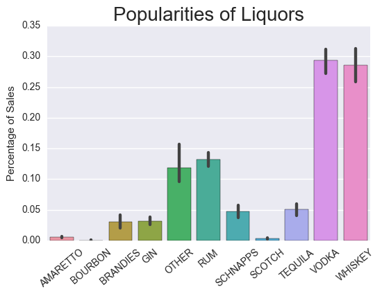
Vodka, Whiskey, and Rum are the top 3 types of liquor. The average items per store for top 10 is 164. Assuming this would be the size of the store, lets multiply the percentages times 164. The ideal mix of liquors, assuming 164 items per store,for a new store should be:
| Rank | Category | Ideal_Mix_Qty |
|---|---|---|
| 0 | VODKA | 49 |
| 1 | WHISKEY | 46 |
| 2 | RUM | 21 |
| 3 | OTHER | 18 |
| 4 | TEQUILA | 9 |
| 5 | SCHNAPPS | 7 |
| 6 | GIN | 6 |
| 7 | BRANDIES | 6 |
| 8 | AMARETTO | 1 |
| 9 | BOURBON | 1 |
| 10 | SCOTCH | 1 |
Plotting the impact of a new store location
We created a barchart of Fraction of Stores that are Liquor Stores by City for the top 10 cities.
Then we plotted the popularity of liquors by category.
Finally, we plotted the impact of entering the market in each of the top 10 cities.
Conclusion
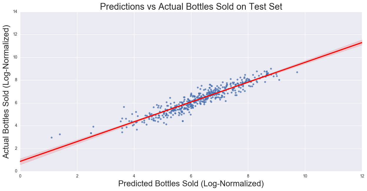
Given the 10% random sample of the Iowa Liquor Sales, the log-normalized Linear Regression Model was used to fit the data to the model. Using the yearly Bottles Sold per each store as the target variables, the predictors Unique Items per Store, Stores per City, Avg Price, Population, and Income were used to fit the model. The correlation and MSE of the data was 0.88 and 0.17, respectively. The model was then used to predict on the test set, and comparing actual Bottles Sold to predicted Bottles Sold 0.87 and 0.19, respectively.
Top 10 Cities are recommended using Average Sales per number of competition, which is stores per city. Since we are interested in the scenario where a new store enters the market. We add 1 to the stores per city and divide Avg Sales by this number. Also assumed was that avg price and bottles sold per city were constant. The following cities are recommended for new markets for a new store location: Mt Vernon, Windsor Heights, Milford, Bettendorf, Iowa City, Mason City, Clinton, Spirit Lake, Cedar Falls, and Coralville. Using the types of Liquor sold (binning them into types), the ideal mix of products to be sold was calculated, which is based on the aggregate of top 10 cities.
Further Analysis can be performed on the brand and size of each type of liquor, as well as the optimal price based on calculated price elasticities.
Hope you enjoyed following along :)
Collaborators: Amish Dalal, Thomas Voreyer